JMeter Result Analysis: The Ultimate Guide

I'm sure you agree that: There are so many ways to collect and interpret JMeter Results, you feel lost.

Well, it turns out after reading this post, you will know 12 different ways to collect and analyze results!

We're going to explore every single possible way to get insightful metrics, including graphs, charts, tables, html reports and more. JMeter is such a complex tool with so many amazing possibilities that it becomes difficult to know what to do.

This ultimate guide about How To Analyze JMeter Results will jump start your JMeter knowledge.

Need professional services?

Rely on our Expertise

Pre-requisites

Installation

This tutorial assumes you already have the following software installed:

• Java 8,
• JMeter 3.3 or above.

During the whole guide, the following Sample JMX is used. This JMX tests our demo application based on a Java JPetstore bundled in a Docker Image.

Understanding JMeter Metrics

JMeter Metrics are widely used in the following section, thus it's better if you're comfortable with their definition:

• Elapsed time: Measures the elapsed time from just before sending the request to just after the last chunk of the response has been received,
• Latency: Measures the latency from just before sending the request to just after the first chunk of the response has been received,
• Connect Time: Measures the time it took to establish the connection, including SSL handshake,
• Median: Number which divides the samples into two equal halves,
• 90% Line (90^th Percentile): The elapsed time below which 90% of the samples fall,
• Standard Deviation: Measure of the variability of a data set. This is a standard statistical measure,

• Thread Name: Derived from the Thread Group name and the thread within the group. The name has the format groupName + " " + groupIndex + "-" + threadIndex where:

• groupName: name of the Thread Group element,

• groupIndex: number of the Thread Group in the Test Plan, starting from 1,

• threadIndex: number of the thread within the Thread Group, starting from 1.

• Throughput: Calculated as requests/unit of time. The time is calculated from the start of the first sample to the end of the last sample. The formula is: Throughput = (number of requests) / (total time).

Interpreting JMeter Metrics

How do you know if a metric is satisfying or awful? Here are some explanations:

• Elapsed Time / Connect Time / Latency: should be as low as possible, ideally less than 1 second. Amazon found every 100ms costs them 1% in sales, which translates to several millions of dollars lost,
• Median: should be close to average elapsed response time,
• XX% line: should be as low as possible too. When it's way lower than average elapsed time, it indicates that the last XX% requests have dramatically higher response times than lower ones,
• Standard Deviation: should be low. A high deviation indicates discrepancies in responses times, which translates to response time spikes.

See, it's pretty easy! Most of the figures should be as low as possible. However, depending on the context, your boss may provide you with expected responses times under a given load. Use them to compute the Apdex of each request:

Apdex (Application Performance Index) is an open standard developed by an alliance of companies. It defines a standard method for reporting and comparing the performance of software applications in computing.

JMeter HeadLess Tests

To run JMeter in headless (non-GUI) mode, which means without any UI, to run load tests use the following command:

jmeter -n -t scenario.jmx -l jmeter.jtl

The command line has the following parameters:

• -n: run in non-GUI mode,
• -t: specifies the path to source .jmx script to run,
• -l: specifies the path to the JTL file which will contain the raw results.

See our blog post How To Optimize JMeter for Large Scale Tests to understand why running in non-GUI mode is vital.

Running the Demo App

To run the demo application on your own computer, you will need:

• An operating system compatible with Docker, See Docker Installation for more information,
• Docker.

To run the JPetstore demo application, simply execute the command-line docker run -d -p 8080:8080 jloisel/jpetstore6.

Open your browser, and navigate to https://localhost:8080/actions/Catalog.action. It should show the JPetstore front page.

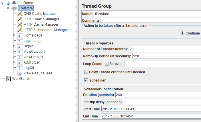
Thread Group Configuration

The following test will be run:

• 20 concurrent thread groups,
• 120 seconds rampup duration,
• 120 seconds peak test duration.

The test will run for a total of 4 minutes with 20 concurrent users peak load.

UI Listeners

JMeter has a number of UI Listeners which can be used to view results directly in JMeter UI:

• View Results as Tree: The View Results Tree shows a tree of all sample responses, allowing you to view the response for any sample.,
• Graph Results: The Graph Results listener generates a simple graph that plots all sample times,
• Aggregate Report: The aggregate report creates a table row for each differently named request in your test,
• View Results In Table: This visualizer creates a row for every sample result. Like the View Results Tree, this visualizer uses a lot of memory,
• Aggregate Graph: The aggregate graph is similar to the aggregate report. The primary difference is the aggregate graph provides an easy way to generate bar graphs and save the graph as a PNG file,
• Generate Summary Results: This test element can be placed anywhere in the test plan. Generates a summary of the test run so far to the log file and/or standard output. Both running and differential totals are shown.

Some listeners have been omitted: these listeners are for debugging purpose only. These listeners help to diagnose scripting issues but are not intended to provide performance metrics, like the following ones:

• Comparison Assertion Visualizer: The Comparison Assertion Visualizer shows the results of any Compare Assertion elements,
• or Assertion Results: The Assertion Results visualizer shows the Label of each sample taken.

As a general rule of thumb, avoid using UI Listeners. They consume a lot of memory. They aren't suitable for real load tests. Some may even trigger and Out Of Memory error with just a few concurrent threads groups running.

Placing Listeners

Depending on the location where the results listener is placed, it collects different metrics. A JMeter results listener collects results from all elements at same level or below. For this reason, it's advisable to place listeners on Test Plan level to collect all thread groups results.

View Results Tree

The View Results Tree is essentially a tool to debug the requests sent and responses received. It's useful to see if the script is running correctly. But, it's not really suitable to view results when many concurrent users are running. It will quickly run out of memory because it keeps all the results in the main memory.

Some metrics are available when clicking on each request like the following:

Thread Name: JPetstore 1-1
Sample Start: 2017-10-06 10:42:09 CEST
Load time: 30
Connect Time: 0
Latency: 29
Size in bytes: 1530
Sent bytes:582
Headers size in bytes: 196
Body size in bytes: 1334
Sample Count: 1
Error Count: 0
Data type ("text"|"bin"|""): text
Response code: 200
Response message: OK

I would suggest to use this listener to:

• Debug the script before scaling the test to a larger number of concurrent users,
• Define baseline performance metrics by running a single thread group for one iteration,
• and/or Use Received Responses to fix / design post processor to extract dynamic parameters.

Aggregate Graph

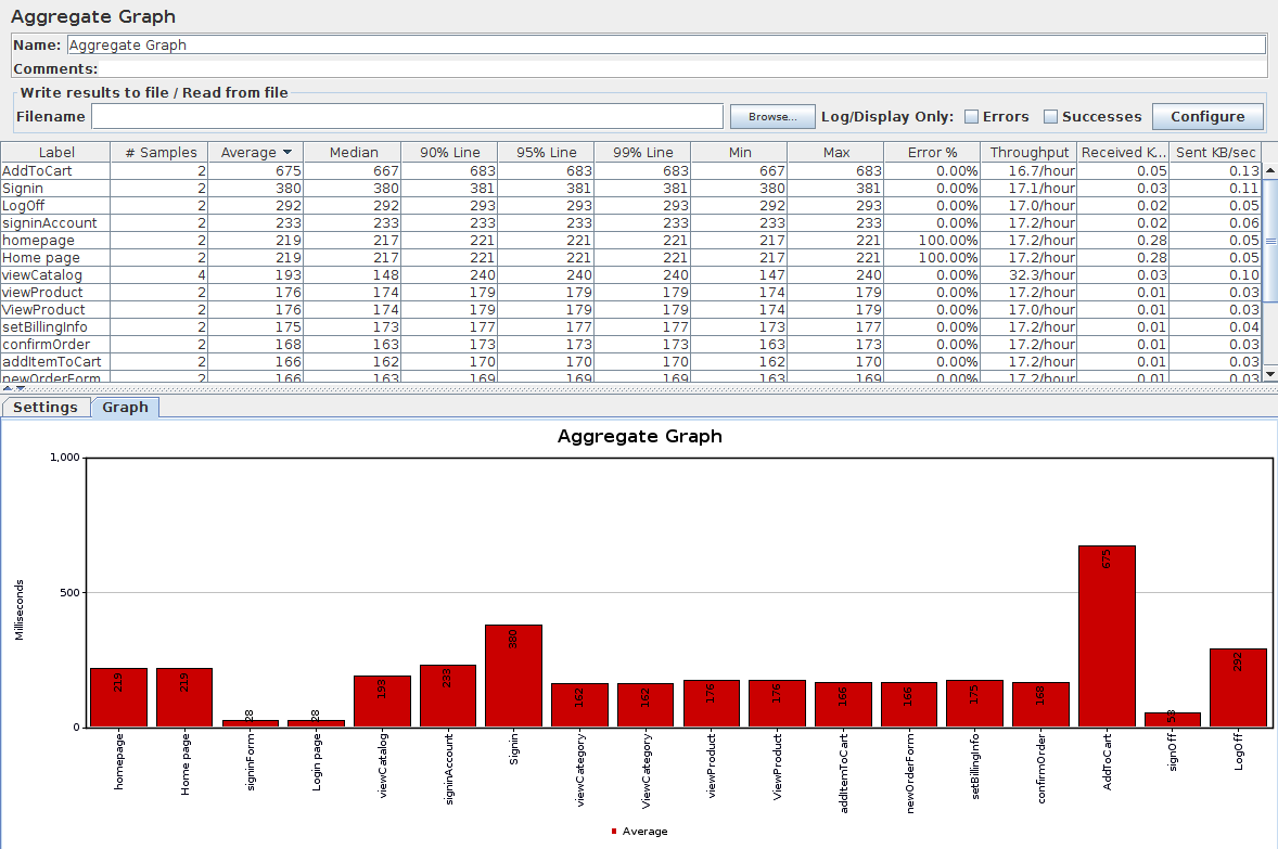
The aggregate graph is an UI Listener which brings some useful test-wide metrics about each request and transaction controller. It also includes a Bar Chart which can be tweaked to fit your needs with many different settings. I must say, there are way too many settings, and even worse, none of these settings are saved in the JMX. You loose them when you close JMeter.

Although, I must admit it's really nice to be able to Export the Graph As PNG and Export Table as CSV for future use in a custom designed report.

The metrics are test-wide, which means you get for example the average response time of a request for the entire test. the available metrics are:

• Label: name of the request,
• # Samples: total number of executions,
• Average: Average Elapsed Time in milliseconds,
• Median: The Median is the value separating the higher half of a data sample, a population, or a probability distribution, from the lower half. For a data set, it may be thought of as the "middle" value,
• 90% Line: 90% Percentile, A percentile (or a centile) is a measure used in statistics indicating the value below which a given percentage of observations in a group of observations fall,
• 95% Line: 95% Percentile,
• 99% Line: 99% Percentile,
• Min: Minimum Elapsed Time,
• Max: Maximum Elapsed Time,
• Errors %: Percentage of errors (errors / (errors + samples) * 100),
• Throughput: Number of samples per second,
• and KB/sec: Network Throughput in KiloBytes/sec.

Like any other UI Listener, I wouldn't recommend using it for real load tests.

Aggregate Report

The aggregate report is very similar to the Aggregate Graph, containing only the metrics table. This listener can be used when running headless load tests (without the UI being launched) because the statistics can be saved in a CSV file for later use. It contains exactly the same metrics as the Aggregate Graph. These metrics can then be used to write a report using Word for example.

Generate Summary Results

JMeter summary Results listener outputs results during the load test in JMeter's console as shown below.

It displays just a few general metrics every few seconds:

Generate Summary Results +      5 in 00:00:07 =    0.8/s Avg:   159 Min:    29 Max:   238 Err:     1 (20.00%) Active: 1 Started: 1 Finished: 0
Generate Summary Results +      7 in 00:00:22 =    0.3/s Avg:   163 Min:    54 Max:   239 Err:     0 (0.00%) Active: 0 Started: 1 Finished: 1
Generate Summary Results =     12 in 00:00:28 =    0.4/s Avg:   161 Min:    29 Max:   239 Err:     1 (8.33%)
Generate Summary Results +     17 in 00:00:25 =    0.7/s Avg:   185 Min:    28 Max:   524 Err:     3 (17.65%) Active: 3 Started: 3 Finished: 0
Generate Summary Results +     32 in 00:00:30 =    1.1/s Avg:   160 Min:    28 Max:   239 Err:     2 (6.25%) Active: 2 Started: 5 Finished: 3
Generate Summary Results =     49 in 00:00:55 =    0.9/s Avg:   169 Min:    28 Max:   524 Err:     5 (10.20%)
Generate Summary Results +     29 in 00:00:30 =    1.0/s Avg:   164 Min:    28 Max:   246 Err:     3 (10.34%) Active: 3 Started: 8 Finished: 5
Generate Summary Results =     78 in 00:01:25 =    0.9/s Avg:   167 Min:    28 Max:   524 Err:     8 (10.26%)
Generate Summary Results +     31 in 00:00:30 =    1.0/s Avg:   165 Min:    28 Max:   242 Err:     2 (6.45%) Active: 2 Started: 10 Finished: 8
Generate Summary Results =    109 in 00:01:55 =    0.9/s Avg:   166 Min:    28 Max:   524 Err:    10 (9.17%)
Generate Summary Results +      4 in 00:00:05 =    0.8/s Avg:   168 Min:   138 Max:   181 Err:     0 (0.00%) Active: 0 Started: 10 Finished: 10
Generate Summary Results =    113 in 00:02:00 =    0.9/s Avg:   166 Min:    28 Max:   524 Err:    10 (8.85%)

These log lines are already output by default when running JMeter in headless mode. JMeter Jenkins Plugin is capable of parsing those lines and output graphs when running JMeter on Jenkins.

Graph Results

JMeter Graphs Results displays line charts for common metrics as well as number figures:

• No of Samples: the number of samples being processed,
• Latest Sample: Latest Elapsed Time in milliseconds,
• Average Elapsed Time: in milliseconds,
• Standard Deviation: in milliseconds,
• and Throughput: in KB/sec.

This results listener is not worth it. The graphs are barely readable. And, as explained in JMeter documentation:

Graph Results MUST NOT BE USED during load test as it consumes a lot of resources (memory and CPU). Use it only for either functional testing or during Test Plan debugging and Validation.

Summary

To summarize, most UI listeners are great for debugging / testing purpose. Don't expect to hit high loads ( >= 500 concurrents users), use them sparingly. These listeners have been designed to quickly get metrics while running load tests inside JMeter UI, for very light loads. (<= 50 concurrent users)

It may be possible to use them even for medium load (100 - 500 concurrent users), but don't expect to run distributed JMeter tests with JMeter UI. It's not the purpose. Remember JMeter is configured with 512MB heap memory by default, which is fairly low. Although you can Increase JMeter allocated memory, it feels coping water out of a boat which doesn't float anymore.

Now that we have tested most of the UI listeners available in JMeter, the question is obviously: Which Listeners can we use when running real load tests ?

Headless Listeners

Headless JMeter Listeners (or non-UI) are specially designed to work when JMeter is run from the command line. Those listeners are those being used when running real load tests, because they use far less memory than UI Listeners. How? These listeners don't keep results in memory, they are mostly in charge of offloading results to another medium.

The existing non-GUI JMeter Listeners are:

• Simple Data Writer: Listeners can be configured to save different items to the result log files (JTL),
• Backend Listener: The backend listener is an Asynchronous listener that enables you to plug custom implementations of BackendListenerClient. By default, a Graphite implementation is provided.

Simple Data Writer

This is the single most useful listener in JMeter. It saves performance metrics according to the configuration inside an external file: the JTL file. JMeter JTL files are the best way to analyze results, but come with a down side: you need another tool to perform data-mining.

There are currently two types of JTL file:

• CSV (default, with or without headers),
• and XML.

The XML files can contain more types of information, but are considerably larger. Therefore, it's recommended to stick to the CSV format. The produced jmeter.jtl contains datas like these:

timeStamp,elapsed,label,responseCode,responseMessage,threadName,dataType,success,failureMessage,bytes,sentBytes,grpThreads,allThreads,Latency,IdleTime,Connect
1507280285885,221,Home page,,"Number of samples in transaction : 1, number of failing samples : 1",JPetstore 1-1,,false,,59592,10154,1,1,50,1,23
1507280286687,29,signinForm,200,OK,JPetstore 1-1,text,true,,1531,582,1,1,29,0,0
1507280286108,29,Login page,200,"Number of samples in transaction : 1, number of failing samples : 0",JPetstore 1-1,,true,,1531,582,1,1,29,580,0
1507280286819,147,viewCatalog,200,OK,JPetstore 1-1,text,true,,3460,11027,1,1,27,0,0
1507280287967,233,signinAccount,200,OK,JPetstore 1-1,text,true,,3719,13270,1,1,55,0,27
1507280286717,380,Signin,200,"Number of samples in transaction : 2, number of failing samples : 0",JPetstore 1-1,,true,,7179,24297,1,1,82,1104,27
1507280292035,162,viewCategory,200,OK,JPetstore 1-1,text,true,,2600,6502,1,1,56,0,26
1507280288201,162,ViewCategory,200,"Number of samples in transaction : 1, number of failing samples : 0",JPetstore 1-1,,true,,2600,6502,1,1,56,3834,26
1507280297083,174,viewProduct,200,OK,JPetstore 1-1,text,true,,2643,6804,1,1,55,0,26
1507280292198,174,ViewProduct,200,"Number of samples in transaction : 1, number of failing samples : 0",JPetstore 1-1,,true,,2643,6804,1,1,55,4886,26
1507280301651,162,addItemToCart,200,OK,JPetstore 1-1,text,true,,2827,6824,1,1,54,0,25
1507280304617,169,newOrderForm,200,OK,JPetstore 1-1,text,true,,3026,6804,1,1,55,0,27
1507280306851,173,setBillingInfo,200,OK,JPetstore 1-1,text,true,,2759,8194,1,1,63,0,28
1507280310018,163,confirmOrder,200,OK,JPetstore 1-1,text,true,,2980,6475,1,1,56,0,26

We'll see later in this guide how we can use the results saved into the JTL file for further processing and drill-down. JTLs are the most powerful way to analyze JMeter results.

Pros:

• JTLs are plain CSV files easy to read,
• Some Web-Based tools are capable of parsing JTL files and render online reports,
• All Raw Results are saved with JTL files.

Cons:

• JTLs are written by each load generator on their disk. Distributed testing requires to bring them back to the controller at the end of the test,
• JTLs can grow large (several GB) and clutter the disk,
• JTLs must be data-mined with tools like Excel to get useful metrics out of them.

Let's see how we can interpret those JTL files.

JTL Analysis with Excel

%APACHE_JMETER_HOME%/extras contains several xsl files which are specially designed to process JTL files in XML format and output nice reports. Seek for the following files:

• jmeter-results-detail-report_21.xsl: Detailed JMeter Report,
• jmeter-results-report_21.xsl: Basic JMeter Report.

The procedure below explains how to get nice reports using those XSL stylesheets and Microsoft Excel.

How to Analyze JTL files with Excel

• Simple Data Writer Listener: Add it to your Test Plan configure it to save the results as XML in the JTL file,

• Run the load test: From APACHE_JMETER_HOME, run the command ./bin/jmeter -n -t jpetstore.jmx -l jmeter.jtl,

Creating summariser <summary>
Created the tree successfully using jpetstore.jmx
Starting the test @ Fri Oct 06 15:03:42 CEST 2017 (1507295022425)
Waiting for possible Shutdown/StopTestNow/Heapdump message on port 4445
summary +     12 in 00:00:18 =    0.7/s Avg:   187 Min:    30 Max:   418 Err:     2 (16.67%) Active: 2 Started: 2 Finished: 0
summary +     27 in 00:00:29 =    0.9/s Avg:   168 Min:    29 Max:   270 Err:     2 (7.41%) Active: 2 Started: 4 Finished: 2
summary =     39 in 00:00:47 =    0.8/s Avg:   173 Min:    29 Max:   418 Err:     4 (10.26%)
summary +     33 in 00:00:31 =    1.1/s Avg:   163 Min:    28 Max:   259 Err:     3 (9.09%) Active: 2 Started: 7 Finished: 5
summary =     72 in 00:01:18 =    0.9/s Avg:   169 Min:    28 Max:   418 Err:     7 (9.72%)
summary +     27 in 00:00:29 =    0.9/s Avg:   165 Min:    29 Max:   246 Err:     2 (7.41%) Active: 2 Started: 9 Finished: 7
summary =     99 in 00:01:47 =    0.9/s Avg:   168 Min:    28 Max:   418 Err:     9 (9.09%)
summary +     14 in 00:00:13 =    1.1/s Avg:   163 Min:    28 Max:   246 Err:     1 (7.14%) Active: 0 Started: 10 Finished: 10
summary =    113 in 00:02:00 =    0.9/s Avg:   167 Min:    28 Max:   418 Err:    10 (8.85%)
Tidying up ...    @ Fri Oct 06 15:05:43 CEST 2017 (1507295143106)
... end of run

• Edit the JTL: add <?xml-stylesheet type="text/xsl" href="PATH_TO_jmeter-results-report_21.xsl"?> after <?xml version="1.0" encoding="UTF-8"?>,
• Save JTL,
• Open Microsoft Excel: then drag'n drop the JTL file inside it.

Please note that it doesn't work with Open Office. Only Microsoft Office is supported.

With the newly available JMeter Report Dashboard, this legacy solution is not so appealing anymore. The report looks old-fashioned compared to the new JMeter HTML report available since JMeter 3.0.

HTML Report DashBoard

The HTML Report Dashboard can be generated at the end of the test using a separate command line. This report is pretty rich and displays many different metrics. For a complete list of all customisable settings, please see Generating Dashboard on JMeter's website.

Once you have a JTL containing all the results, run:

./bin/jmeter -g JTL_FILE -o OUTPUT_FOLDER

Where:

• -g JTL_FILE: relative or full path to the JTL file. Example: jmeter.jtl,
• -o OUTPUT_FOLDER: the folder in which the HTML report should be written.

The command-line execution may take a while depending on the JTL file size. Once finished, no error should be displayed within the terminal. The report is ready in the given output folder.

Pros:

• HTML Report is easy to generate,
• Graphs and Tables are well designed,
• You can select / deselect requests and/or transactions on each graph.

Cons:

• Too Many customisation settings, where to start?
• The report cannot be fully customized by adding text, images and more. It's a static report.

Since JMeter 3.0, HTML Report Dashboard is a huge step forward simplifying JMeter test result analysis.

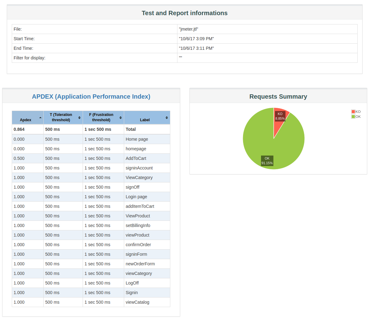
The Report Summary contains the following information:

• Test start time and end time,
• APDEX scores for every single request and container,
• A pie chart named Requests Summary which gives the proportion of Successful / Failed samples.

The Statistics table provides global test statistics for every single request which has been executed:

• Executions: Number of hits and errors,

• # Samples: Total Number of samples executed,

• KO: Total Number of samples failed to execute,

• Errors %: Percent of errors,

• Response Times (ms): Response times in milliseconds,

• Average: Average Elapsed Time,

• Min: Minimum Elapsed Time,
• Max: Maximum Elapsed Time,
• 90^th pct: 90^th Percentile,
• 95^th pct: 95^th Percentile,
• 99^th pct: 99^th Percentile,

• Throughtput: Number of hits per second,

• Network: throughput in KB/sec

• Received: KB received per second,
• Sent: KB sent per second.

The lines can be ordered by any of the statistic above, making it easy to find requests that cause bottlenecks. Order Requests by decreasing Average, you should see the slowest request being first in the statistics table.

The errors table give more details about the errors encountered during the load test. For each type of error, you will see:

• Number of errors: how many errors occured,
• % in errors: percentage of requests in error,
• % in all samples: Percentage of errors compared to total number of samples.

This chart displays the average response time of each transaction over the course of the entire test. Sadly, if you have a lot of transactions, the graph may look cluttered because all the transactions are displayed on it.

There are many other graphs available:

• Throughput:

• Hits Per Second (excluding embedded resources): number of hits per second over time,

• Codes Per Second (excluding embedded resources): HTTP Codes per second over time (200 OK, 500 Internal Error etc.)
• Transactions Per Second: transactions (related to Transaction Controller) per second over time,
• Response Time Vs Request: The response time compared to requests per second,

• Latency Vs Request: Latency compared to requests per second,

• Response Times:

• Response Time Percentiles: Elapsed Time per percentile in 10% increments,

• Response Time Overview: Gives the percent of requests per Apdex Range (Satisfying, Tolerating and Frustrating),
• Time Vs Threads: Elapsed Time per Active Threads, to see how the elapsed time degrades when load increases,
• Response Time Distribution: how Elapsed Time is spread between Min and Max elapsed time.

The HTML report is clearly a good step to catch up with some expensive tools like LoadRunner or NeoLoad. Sure, it could have been way more customisable to taylor a report which fits your needs. Anyway, it's a huge leap forward in improving JMeter test results analysis compared to the integrated UI listeners.

Considering JMeter is an open-source load testing tool, available for free, I'm impressed to see how many tools there are to analyze test results. And we're not even finished yet!

Backend Listener

JMeter's Backend Listener allows to plug an external database to store test results and performance metrics.

In this section, we're going to combine several open-source tools to collect and visualize JMeter results in real-time:

• InfluxData: database used as a temporary metrics storage to store performance metrics,
• Grafana: Grafana is an open-source platform for time series analytics, which allows you to create real-time graphs based on time series data,
• JMeter's Backend Listener: the backend listeners collect JMeter metrics and sends them to the temporary metrics storage.

Exposed Metrics

JMeter sends metrics the the time-series database. The list below describes the metrics being available.

• Thread Metrics:

• ROOT_METRICS_PREFIX_ test.minAT: Minimum active threads,

• ROOT_METRICS_PREFIX_ test.maxAT: Maximum active threads,
• ROOT_METRICS_PREFIX_ test.meanAT: Mean active threads,
• ROOT_METRICS_PREFIX_ test.startedT: Started threads,

• ROOT_METRICS_PREFIX_ test.endedT: Finished threads.

• Response Time Metrics:

• ROOT_METRICS_PREFIX__ SAMPLER_NAME .ok.count: Number of successful responses for sampler name,

• ROOT_METRICS_PREFIX__ SAMPLER_NAME .h.count: Server hits per seconds, this metric cumulates Sample Result and Sub results (if using Transaction Controller, "Generate parent sampler" should be unchecked),
• ROOT_METRICS_PREFIX__ SAMPLER_NAME .ok.min: Min response time for successful responses of sampler name,
• ROOT_METRICS_PREFIX__ SAMPLER_NAME .ok.max: Max response time for successful responses of sampler name,
• ROOT_METRICS_PREFIX__ SAMPLER_NAME .ok.avg: Average response time for successful responses of sampler name,
• ROOT_METRICS_PREFIX__ SAMPLER_NAME .ok.pct_PERCENTILE_VALUE: Percentile computed for successful responses of sampler name. There will be one metric for each calculated value,
• ROOT_METRICS_PREFIX__ SAMPLER_NAME .ko.count: Number of failed responses for sampler name,
• ROOT_METRICS_PREFIX__ SAMPLER_NAME .ko.min: Min response time for failed responses of sampler name,
• ROOT_METRICS_PREFIX__ SAMPLER_NAME .ko.max: Max response time for failed responses of sampler name,
• ROOT_METRICS_PREFIX__ SAMPLER_NAME .ko.avg: Average response time for failed responses of sampler name,
• ROOT_METRICS_PREFIX__ SAMPLER_NAME .ko.pct_PERCENTILE_VALUE: Percentile computed for failed responses of sampler name. There will be one metric for each calculated value,
• ROOT_METRICS_PREFIX__ SAMPLER_NAME .a.count: Number of responses for sampler name (sum of ok.count and ko.count),
• ROOT_METRICS_PREFIX__ SAMPLER_NAME .a.min: Min response time for responses of sampler name (min of ok.count and ko.count),
• ROOT_METRICS_PREFIX__ SAMPLER_NAME .a.max: Max response time for responses of sampler name (max of ok.count and ko.count),
• ROOT_METRICS_PREFIX__ SAMPLER_NAME .a.avg: Average response time for responses of sampler name (avg of ok.count and ko.count),
• ROOT_METRICS_PREFIX__ SAMPLER_NAME .a.pct_PERCENTILE_VALUE: Percentile computed for responses of sampler name. There will be one metric for each calculated value. (calculated on the totals for OK and failed samples).

The following constants are:

• ROOT_METRICS_PREFIX_: root metrics prefix. There is none when using InfluxBackendListenerClient,
• SAMPLER_NAME: name of the sample within the JMX script,
• PERCENTILE_VALUE: 90, 95 or 99 by default. Depends on the backend listener configuration.

InfluxDB Setup

We're going to download and install influxDB:

• Download InfluxDB,
• Install InfluxDB, here is the setup for Ubuntu using A Debian package:

ubuntu@desktop:~$ wget https://dl.influxdata.com/influxdb/releases/influxdb_1.3.6_amd64.deb
ubuntu@desktop:~$ sudo dpkg -i influxdb_1.3.6_amd64.deb 
Selecting previously unselected package influxdb.
(Reading database ... 264577 files and directories currently installed.)
Preparing to unpack influxdb_1.3.6_amd64.deb ...
Unpacking influxdb (1.3.6-1) ...
Setting up influxdb (1.3.6-1) ...
Created symlink from /etc/systemd/system/influxd.service to /lib/systemd/system/influxdb.service.
Created symlink from /etc/systemd/system/multi-user.target.wants/influxdb.service to /lib/systemd/system/influxdb.service.
ubuntu@desktop:~$

InfluxDB setup can vary depending on your operating system. Please see InfluxDB Installation for more information.

• Start influxdb service by running ubuntu@desktop:~$ sudo service influxdb start,
• Run the command influx in terminal to connect to the database,
• Create JMeter's database:

ubuntu@desktop:~$ influx
Connected to https://localhost:8086 version 1.3.6
InfluxDB shell version: 1.3.6
> show databases
name: databases
name
----
_internal
> CREATE DATABASE jmeter
>

Great, InfluxDB is up and running!

Grafana Setup

Grafana is the dashboard which will allow use to visualize the metrics sent by JMeter to the InfluxDB Database.

• Download Grafana and install it (Ubuntu setup here):

wget https://s3-us-west-2.amazonaws.com/grafana-releases/release/grafana_4.5.2_amd64.deb 
sudo dpkg -i grafana_4.5.2_amd64.deb 

• Browse to https://localhost:3000 to open grafana dashboard. Use admin as login and password.

• Select Add DataSource option,

• Then configure DataSource with the following settings:

• Name: influxdb, any name should work,

• Type: InfluxDB, as we connect to an InfluxDB Database,
• Url: https://localhost:8086/,
• Access: Direct, because it's direct connection to the database,
• Database: jmeter, the previously created database.

BackendListener Setup

Now, let's add a backend listener to our Test Plan:

• Open JMeter, then open the sample JMX Script,
• Right-click on the test plan, and select Add > Listener > Backend Listener,

• Configure the backend listener with the following settings:

• influxdbMetricsSender: implementation class for sending metrics to InfluxDB. As of JMeter 3.2, InfluxDB is available without the need to add any additional plugin,

• influxDbUrl: InfluxDB database url, the url of InfluxDB in format: https://[influxdb_host]:[influxdb_port]/write?db=[database_name]. As we have created the jmeter database and we are running it on local machine with default port then in our case url will be: https://127.0.0.1:8086/write?db=jmeter
• application: name of the application. This parameter allows to group metrics by name, thus allowing to use the same database for multiple different tests,
• measurement: name of measurement that will be stored in InfluxDB (text-based line InfluxDB internal protocol to store metrics). Use default ‘jmeter’ for that property,
• summaryOnly: put false if you want to keep detailed metrics in the database,
• samplesRegex: allows to filter results being stored by sampler name,
• percentiles: defines the percentiles being processed and sent to InfluxDB, 90;95;99 by default,
• testTitle: we use JPetstore here,
• eventTags: a list of tags which will be stored in the ‘events’ measurement of InfluxDB.

Running a test

Now, it's time to run the test within JMeter. Either launch the test in GUI or non-GUI mode.

To check that the results are properly sent to InfluxDB, run the following command:

curl 'https://localhost:8086/query?pretty=true' --data-urlencode "db=jmeter" --data-urlencode "q=SHOW SERIES"
{
    "results": [
        {
            "statement_id": 0,
            "series": [
                {
                    "columns": [
                        "key"
                    ],
                    "values": [
                        ...
                        [
                            "events,application=jpetstore,title=ApacheJMeter"
                        ],
                        [
                            "jmeter,application=jpetstore,responseCode=0,responseMessage=Number\\ of\\ samples\\ in\\ transaction\\ :\\ 1\\,\\ number\\ of\\ failing\\ samples\\ :\\ 1,transaction=Home\\ page"
                        ],
                        ...
                    ]
                }
            ]
        }
    ]
}

The returned Json document should contain several values. Let's configure a Grafana dashboard to visualize Hits/sec.

Creating a JMeter Dashboard

• Select Create your first dashboard,
• Select Graph,
• Click on Panel Title then Edit,

• Now, let's configure the metrics:

• Data Source: select the InfluxDB data-source previously configured,

• FROM: default jmeter, WHERE application = jpetstore,
• SELECT: field count mean(), which is the average number of samples,
• GROUP BY: time($_interval) fill(linear), to get a beautiful line chart,
• FORMAT AS: Time Series.

It should produce the graph shown on the screenshot below.

Prometheus Listener

Prometheus is, like InfluxDB, another time-series database but unlike InfluxDB JMeter does not natively support integration with Prometheus and therefore we will be using the really good jmeter-prometheus-plugin created by Jeff Ohrstrom.

This plug-in exposes metrics captured in JMeter through an API for Prometheus to scrape from, the principles of how Prometheus scrapes data can be found on their website, here.

Exposed Metrics

Now the subject of the metric types that Prometheus captures is one this is defined here.

There are 4 metrics, and each will form part of our example test, these are:

• Counter
• Gauge
• Histogram
• Summary

The below table shows which measures from JMeter can be displayed with the different Metrics Types, notice that there is no coverage for Gauge at present.

Measure	Histogram	Summary	Counter	Gauge	Success Ratio
Response time	x	x
Response size	x	x
Latency	x	x
Idle time	x	x
Connect time	x	x
Count total			x
Failure total			x
Success total			x
Success ratio					x

Prometheus Setup

Prometheus is an ideal candidate for data analysis from tools such as JMeter due to the way it stores and manages data, from the Prometheus website.

Prometheus fundamentally stores all data as time series: streams of timestamped values belonging to the same metric and the same set of labeled dimensions. Besides stored time series, Prometheus may generate temporary derived time series as the result of queries.

There is much more information on Prometheus and how it works on its website, here.

Download Prometheus from here.

Once downloaded and uncompressed you will see these files:

The first thing we need to do is to update the prometheus.yml file

We need to add

  - job_name: 'jmeter'
    # metrics_path defaults to '/metrics'
    # scheme defaults to 'http'.
    static_configs:
    - targets: ['localhost:9270']

To the end of the file so that it now looks like

What we have added is the location of the JMeter /metrics API which was defined in the properties section we outlined in the JMeter section above.

Property	Default	Description
prometheus.port	9270	The port the http server will bind to
prometheus.ip	127.0.0.1	The ip the http server will bind to. Containers may need 0.0.0.0

If we now start our local Prometheus instance using this command

./prometheus.exe --config.file=prometheus.yml

Prometheus is now running on our local host on port 9090. Meaning that we can now enter this URL into a browser https://localhost:9090 to see our Prometheus instance running:

Prometheus does come with some graph capability but nowhere near as good as Grafana and therefore we will move on to the Grafana installation next, but we will come back to Prometheus later.

Grafana Setup

We have already discussed how to set up Grafana but we need to add a data source to visualise data from our local Prometheus instance.

From within your Grafana instance select Data sources from the Configuration option

Select Prometheus from the data source list

Enter https://localhost:9090 into the URL field, it looks like it is populated but it is not, you need to overtype the value explicitly.

Select Save & test at the bottom of the page

Our data source is now set up

We will leave Grafana for now but will return later once we have some data.

Prometheus Listener Setup

From the JMeter Plugins manager install the Prometheus Listener Plugin.

We will come back to building the test after we have gone through the Prometheus and Grafana setup but before we move on there are several properties that can be overridden and its worth looking at these.

The properties are defined on the GitHub README for this plugin, they are:

Property	Default	Description
prometheus.port	9270	The port the http server will bind to
prometheus.ip	127.0.0.1	The ip the http server will bind to. Containers may need 0.0.0.0
prometheus.delay	0	The delay (in seconds) the http server will wait before being destroyed
prometheus.save.threads	true	True or false value to save and collect jmeter thread metrics
prometheus.save.threads.name	jmeter_threads	The name of the metric describing jmeter threads
prometheus.save.jvm	true	Collect metrics from the JVM

If you want to override these then you simply add them to your JMeter user.properties file with the values you want to use.

We are going to configure a Prometheus listener and set it to output response times in Histogram and Summary format, Counters for transactions (successful, unsuccessful and total) and a Success Ratio counter.

As the Response Size, Latency, Idle Time and Connect Time all display data in a similar way to response time we will not cover these but the way we will visualise data for these is consistent with Response Time.

Let’s look at the Prometheus Listener

The Name filed is a label that we will see in Grafana when we come to visualise the data with the Help field an explanation of what we are capturing.

The Label field has to be populated with either:

• Label is a keyword. In JMeter it means the name of the sampler

• Code is a keyword. It's the response code of the result

• JMeter variables can be used here, so for example if you wanted to include a variable you defined as ${my_variable} then in the labels field you could for example use label,code,my_variable

The types determine how the data will be output and measured and the Buckets or Quartiles being how the values will be compartmentalised so for our Response Time Histogram we are collecting data into 1000ms, 3000ms and 5000ms buckets; if for example your response time requirements stated that 2000ms was the maximum response time for a particular request then you could just put 1000 in this field.

The Response Time Summary sees us looking at response times at the 50% percentile (the Median), the 75^th, 90^th and 95^th percentiles.

The Listen to column allows you to choose between samples or assertions and the Measuring field allows you select what value from JMeter you want to capture, the definitive list is in the measures table above.

We can now look at running our test, we have set the Loop Count to be infinite and we have 50 Threads, before we start we are going to change one of the values in our user.properties file.

We are going to uncomment the setting that outputs the JVM values to Prometheus and set it to false, while useful and is something you should consider enabling as you can visualise this data in Grafana as well, it does make the /metrics API quite noisy and its easier to discuss when this is disabled.

Running a Test

Let’s create a Test Plan to allow us to demonstrate how we can configure the jmeter-prometheus-plugin.

The JMeter project used in this blog post can be found here.

The plugin comes with a listener and a config element, and we will look at both in our example test.

We start by creating a test with a dummy sampler.

We have given the samplers a Response Time that will be a random value between 50 and 5000, the reason we want to give a wide range is so we can demonstrate how response times can be captured and aggregated into buckets and quartiles which is a fundamental principle of how data is aggregated in Prometheus and Grafana.

If you remember the Prometheus Listener outputs to our localhost on port 9270:

Property	Default	Description
prometheus.port	9270	The port the http server will bind to
prometheus.ip	127.0.0.1	The ip the http server will bind to. Containers may need 0.0.0.0

And we configured Prometheus to scrape data from this location

So, while the test is running if we access this URL, we can see the data being output. For information if the test is not running this URL is unavailable.

We can see our data with the name value we gave it in the Listener being produced.

Notice the values at the bottom where jmeter_threads captures the number of users running, this is one of the configurable values in the user.properties file that we can set should you want to call the label something else.

The Config Element outputs data in the same way as the ones we have discussed and the subtle differences between what data can be captured are addressed in the GitHub README.

Creating a JMeter Dashboard

So, we have generated data, which has been scaped by Prometheus and now should be available to visualise in Grafana.

If we go to Grafana and select Create Dashboard we can start adding Panels.

When you select Add Panel you are presented with the ability to grab the data you have just generated and do something meaningful with it.

Make sure you have you Prometheus connection set as the Data source and if you start typing the name value that we used in the Listener you should see the data we sent, and scaped by Prometheus available in Grafana.

The object of the post is to show you the building blocks needed to get your data from JMeter to Grafana and we have done that, to understand Grafana and how you can manage your data effectively is something you will need to explore for yourself however, we have created some visuals that we will show below along with the queries we used to produce them.

Transactions < 1000ms

octoperf_sampler_one_histogram_bucket{le="1000.0"} / ignoring(le) octoperf_sampler_one_histogram_count

Percentile Ratio

octoperf_sampler_one_summary

Successful Requests

octoperf_sampler_one_success_ratio_success / octoperf_sampler_one_success_ratio_total

Response Times Percentiles Over Time

octoperf_sampler_one_summary

Transaction Per Second

rate(octoperf_sampler_one_total_count[1m])

Custom Reporting with Database

Outside of using listeners that write to conventional reporting technologies there are ways to create nice reports from your local machine in a similar way that the Simple Data Writer section talks about.

There are many tools that have already been discussed and many organisations have these available for your use, however getting data into these tools is sometime problematic and their benefits do not always justify any extra costs.

When you are busy and have deadlines sometimes all you want to do is quickly analyse your results and move on because ultimately getting a well performing application is your goal.

We have looked in another blog post about reading data from a database to support your performance testing. Using techniques defined in this post we are going to show you a quick way of producing nice dashboards and tables from your .jtl files.

The Benefits

Whether you run your performance tests in pipelines or from a load injector or even from your local this little trick to quickly and neatly generate results will help with your analysis. You will be able to generate results with no additional overhead once set up and will allow you to produce some nice visualisations.

It allows you to compare sets of results easily and consistently using data generated from your performance tests using open source and community edition solutions meaning there is no cost associated.

As there is a database in this solution your data can be easily stored for an indefinite period of time should you want to keep it and refer back to it.

The Solution

The solution involves using a SQLite database and a local installation of Grafana. It could however be easily expanded to use any database type and you could use your organisations version of Grafana if you use one for other reporting purposes.

The solution is deliberately simple and easy to use as, and we have already touched on this, sometimes all you want to do is produce quick and easy results and continue testing.

The JMeter projects used in this blog post can be found here: Dummy test and Insert DB.

Installing a Local Database

Download SQLite DB from here.

You will need a pre-compiled binary depending on your operations system.

Unzip and set your $PATH to include its location

From the command line let’s create a database using this command.

./sqlite3 OctoPerfResultsDB.db

And then open the database using this command.

.open OctoPerfResultsDB.db

We now have a dummy database ready to write our results into.

Generating Results

Before we move onto the results analysis, we need to create a JMeter test that will generate some dummy results and for the purposes of simplicity we will hardcode the values.

We will create a simple Test Plan with a single Thread Group and 5 Dummy Samplers.

We have added a Simple Data Writer to the test as this is the simplest way to write the results to a flat file.

Notice we have set the extension of the file to be .csv.

If we execute our test, we can see that a .csv file is produced that contains our results.

We are now going to look at how we can read these results into our database.

For the purposes of this post, we are going to create another JMeter test to copy the data, but you could just as easily add this to the data generation test as a teardown ThreadGroup.

The test looks like this and is a single JSR223 Sampler executed by a single thread.

In order to run this test we are going to need the SQLite JAR file which can be downloaded from here and then should be copied to the /lib folder of your JMeter directory.

The JSR223 Sampler is doing all the work here so let’s look at it in more detail, the order we will look at the code is not the order it is written in but it makes more sense to explain it this way.

/* Connect to database */
def connectToDatabase() {
    def url = "jdbc:sqlite:OctoPerfResultsDB.db"
    def user = ""
    def password = ""
    def driver = "org.sqlite.JDBC"
    def sqlConnection = Sql.newInstance(url, user, password, driver)    
    return sqlConnection
}

We are creating a function called connectToDatabase() and assigning this to an object.

Change the URL to point to your local copy of the database you created in the steps above with any relative or absolute path necessary.

We are now going to look at a couple of helper methods that will create the results table and populate the data from the .csv file.

/* Build results table */
def createResultsTable(columnName, sqlConn){
    def createTableQueryString

    // Iterate the columns
    columnName.eachWithIndex{value,index->
        // Create the results table
        // Boiler plate stuff
        if(index == 0) {
            createTableQueryString = "CREATE TABLE OctoPerfResults (" + value + " Integer, "
        }
        else {
            if (index == (columnName.size() - 1)) {
                createTableQueryString += value + " VarChar)"
            }
            else {
                if(value == "elapsed") {
                    createTableQueryString += value + " Integer, "
                }
                else {
                    createTableQueryString += value + " VarChar, "
                }
            }
        }
    }

    // Create the table with .csv columns
    sqlConn.execute createTableQueryString
}

The first method reads the column headings from the .csv file and builds a table based on these headings, all column values are set to Varchar with the exception of the first column which is the timestamp field and the elapsed field which are set to Integer.

If you want to perform maths calculations on any of these columns then they need to be set to Integer.

We have again hardcoded the table name we are creating to OctoPerfResults but you can use a variable or property if you wish and would be better for creating multiple result sets.

The second method adds data to the table we created in the first method.

/* Add data to table */
def addResultsToTable(columnName, columnValues, sqlConn){
    def addToTableQueryString

    // Iterate the columns
    columnName.eachWithIndex{value,index->
        // Create the results table
        // Boiler plate stuff
        if(index == 0) {
            addToTableQueryString = "INSERT INTO OctoPerfResults (" + value + ", "
        }
        else {
            if (index == (columnName.size() - 1)) {
                addToTableQueryString += value + ")"
            }
            else {
                addToTableQueryString += value + ", "
            }
        }
    }

    // Iterate the value
    columnValues.eachWithIndex{value,index->
        if(index == 0) {
            addToTableQueryString += " VALUES ('" + value.substring(0, (value.length() -3)) + "', "
        }
        else {
            if (index == (columnName.size() - 1)) {
                addToTableQueryString += "'" + value + "')"
            }
            else {
                addToTableQueryString += "'" + value + "', "
            }
        }   
    }
    // Insert into the results table
    sqlConn.execute addToTableQueryString
}

You will notice that we trim the last 3 characters from the timestamp value

if(index == 0) {
    addToTableQueryString += " VALUES ('" + value.substring(0, (value.length() -3)) + "', "
}

This is because JMeter output is an epoch time in milliseconds and Grafana requires the timestamp to be an epoch time in seconds.

We then use these methods which we iterate over the file we have output from JMeter in our first test.

// Connect to the DB
    def sqlConn = connectToDatabase()

    // Get the file
    File file = new File("OctoPerfResults.csv")

    // Iterate the file
    // Set some variables
    def line
    def lineNo=0
    String[] columnName
    String[] columnValue

    // Iterate file with closure
    file.withReader { reader ->
       while ((line = reader.readLine()) != null) {
        // Increment the lineNo count
        lineNo++
        // Line 1 contains the table headers
        if(lineNo==1) {
            // Split the line to get the column headings
            columnName = line.split(",")
            // Create the results table
            createResultsTable(columnName, sqlConn)
        }
        else {
            columnValue = line.split(",")
            // The remainder of the lines need to be added to the table 
            addResultsToTable(columnName, columnValue, sqlConn)
        }
       }
    }

    // Close the connection
    sqlConn.close()

Populating the Database

Now we have created our tests let’s execute them and look at the results.

We have already executed the first test and created the .csv file, if we now run the second test we will see the data added to the database.

If we run this command against our database.

.tables

We can see we have a table called OctoPerfResults.

We have now replicated our output file into a database.

View in Grafana

Once you have logged on, we need to add the SQLite plugin to Grafana so we can connect to our database.

Select the plugin option from the configuration menu.

Search for and install the SQLite plugin.

If we now select Data sources we can add our local database.

Now we are connected to our database we can quite easily create some nice visualisations with our data.

Let’s start with a simple table.

Add a new panel to a dashboard and let’s look at how we can construct a query.

We are going to select Table as the type of visualisation and we are going to use this query to get our data.

select label, count(label) as samples, min(elapsed) as min, avg(elapsed) as average, max(elapsed) as max from OctoPerfResults where responseCode = 200 group by label;

We are effectively going to get the label, sample count, min, average and max from our database and group by the label where we have a 200 response.

If we save this, we can see that our SQL query results are now presented in our Grafana dashboard.

Remember to select the correct timeframe in Grafana for your results as otherwise the table will be empty.

We can also create a timeseries graph, let’s add another panel to the dashboard.

This time we will select Time series as the type of visualisation and we are going to use this query to get our data.

Select timeStamp, label as metric, elapsed as value from OctoPerfResults order by timeStamp;

Before we can display our time series graph, we need to add the tag that indicates which column holds the time series data which in our case is the timestamp column.

We can see that time and ts are already created so we have just added one called timestamp.

If we save this, we can see that our SQL query results are now presented in our Grafana dashboard.

Remember to select the correct timeframe in Grafana for your results as otherwise the graph will be empty.

We have now created 2 very quick visualisations from our JMeter output.

Additional Considerations

This is your database and you can keep as much data as you want or truncate or drop the database tables you create with your results.

You can make the SQL as complex as you want to get the data you want and calculating percentiles and grouping data or even joining tables is straightforward.

What we have shown here is a good starting point, but you can display complex data joins and comparison in you results whilst making the solution very quick and efficient.

NovaTec APM Dashboard

Configuring a grafana dashboard yourself is a tedious and difficult task, especially if you have no extended knowledge in querying metrics. They published a pre-configured JMeter Load Test Dashboard.

This dashboard only works with the following backend listener plugin: JMeter InfluxDB Writer

Install JMeter InfluxDB Writer

• Download the plugin from JMeter InfluxDB Writer Download Page,
• Copy the plugin JMETER_HOME/lib/ext,
• Restart JMeter.

Create Dedicated Database

This setup requires a separate database:

• Create new database in InfluxDB named novatec using the following command:

ubuntu@desktop:~$ curl -i -XPOST https://localhost:8086/query --data-urlencode "q=CREATE DATABASE novatec"
HTTP/1.1 200 OK
Connection: close
Content-Type: application/json
Request-Id: b04edfe5-acd4-11e7-8647-000000000000
X-Influxdb-Version: 1.3.6
Date: Mon, 09 Oct 2017 09:31:54 GMT
Transfer-Encoding: chunked

{"results":[{"statement_id":0}]}

Configure JMeter InfluxDB Writer

• Open JMeter, then open the sample JMX Script,
• Right-click on the test plan, and select Add > Listener > Backend Listener,

• Configure the backend listener with the following settings:

• testName: jpetstore,

• nodeName: Test-Node,
• influxDBPort: 8086,
• influxDBUser: jmeter,
• influxDBPassword: none,
• influxDBDatabase: novatec.

Let other settings with default settings.

Create new Data-Source Novatec in Grafana

• Create a new datasource mapped on the database novatec.

Import Novatec Dashboard

Please follow the documentation explaining how to import a Grafana Dashboard in details.

• Open Grafana,
• Select Import new Dashboard,
• Enter ID 1152 which is the ID of the Novatec Dashboard,
• Select the data-source pointing the the novatec database.

You should be able to see animated graphs in the dashboard.

This dashboard offers many interesting metrics through graphs, pie-charts and more:

• Active Users: currently running threads,
• Overall Throughput: Operations per second,
• Success Rate: percentage of requests which have succeeded,
• Request Count: total number of requests executed,
• Error Rate: percentage of requests which have failed,
• Metrics Overview: a table displaying all the metrics, one line per request,
• and more!

InfluxDB Studio

InfluxDB Studio is a UI management tool for InfluxDB. It runs on Windows and allow to administer InfluxDB databases using a user-friendly UI.

Recommended Setup

We strongly recommend using the NovaTec plugin combined with the NovaTec JMeter Dashboard. It provides an out-of-the-box dashboard with many interesting metrics, ready to use. Configuring Grafana by yourself can be difficult and requires knowledge about how InfluxDB queries work.

Saas JMeter Solutions

As we have seen, a complete working setup using the BackendListener can take quite a bit of time to setup. And we're not even talking about maintenance and updates. This is why Cloud solution like OctoPerf, Blazemeter or Flood.io are emerging.

These Saas tools provide a facility to run JMeter tests and collect metrics. Each tool has its own reporting system based on proprietary technologies. We're going to explore each tool here and compare their reporting capabilities. The goal is to get an overview of the reporting capabilities of each JMeter Cloud Solution.

Each tool will be used to run the same test:

• 20 concurrent users,
• 10 min test duration,
• From any location available with a free account.

Please keep in mind that we're trying to be as objective as possible. There are many other tools on the market enabling JMeter results analysis. As a result, we selected only the most popular tools.

Blazemeter

Blazemeter is the first tool which came on the market to allow users to scale their load tests in the cloud. Blazemeter is an american company founded by Alon Girmonsky in December 2011.

Summary Report

The summary report provides the following statistics:

• Max Users: maximum number of concurrent users,
• Avg Throughput: hits per second,
• Errors %: percentage of errors,
• Average Response Time: average response time in milliseconds,
• 90% Response Time: 90% Percentile response time,
• Average Bandwidth: average KiB per second during the test.

It includes two graphs:

• Load Graph: displays hits/sec, errors/sec and concurrent users curves,
• Response Time Graph: displays concurrent users and average response time curves.

The summary is static: metrics cannot be added or removed.

TimeLine Report

The timeline report provides a huge graph whose curves can be customised. Transactions can be individually selected and plotted. It's a little bit sad that the samplers hierarchy isn't kept: all transactions and requests are within a single list. The timeline can get quite messy if many requests are drawn simultaneously.

Request Stats

The request stats provides a table which contains the global statistics for each transaction or request. The following statistics are available:

• # Samples: number of samples,
• Avg Response Time (ms): Average Elapsed Time in milliseconds,
• 90^th line (ms): 90% centile on Elapsed Time in milliseconds,
• 95^th line (ms): 95% centile on Elapsed Time in milliseconds,
• 99^th line (ms): 99% centile on Elapsed Time in milliseconds,
• Min Response Time (ms): Minimum Elapsed Time in milliseconds,
• Max Response Time (ms): Maximum Elapsed Time in milliseconds,
• Average KiB/sec: Network Throughput (download) in KiloBytes per second,
• Error Percentage: Percent of hits in error.

The whole table can be downloaded as a CSV file for external processing. Statistics can be filtered by time.

Errors

This report displays all errors received during the test run, categorized by labels (pages) and error types.

JMeter Logs

JMeter logs per engine are available. Logs can be downloaded or viewed within the browser directly.

Original Test Config

This section is a reminder of the original test configuration.

Executive Summary

The executive summary is a printable version of the test report. It contains everything from the previous sections (Summary, TimeLine and more).

Flood

Flood is a Blazemeter challenger. This Australian company has been founded in September 2013 by Ivan Vanderbyl and Tim Koopsman. They offer pretty much the same features as BlazeMeter: upload your JMX script, run the test and analyze results.

TimeLine

The TimeLine gives an overview of the test result metrics. you can draw a single transaction metrics by selecting it in the table below.

JMeter Logs

JMeter logs can be viewed live while the test is running. The logs can be downloaded at the end of the test.

Request Details

By selecting a single request or transaction, you gain access to a sub-report which gives numerous metrics about that transaction. (Average, Minimum, Maximum, Standard Deviation, Centiles, passed vs failed and more) A few requests and responses are also stored at some random points during the load test.

Miscellaneous

The metrics can be downloaded as a CSV file for external processing.

OctoPerf

OctoPerf is a French load testing company founded in September 2016. OctoPerf's reporting system is a modular system designed which can be customized. Any of the report items below can be rearranged, thus making the reporting system dynamic. The report is pre-configured with certain report items. Items can be added or removed as needed.

For more information, please read the documentation on Report Items.

Test Summary

The test summary displays details about the test configuration like:

• Test Duration,
• Number of concurrent user,
• Geographical location used,
• and more.

Statistics Summary

Statistics summary provides test wide statistics. The following settings can be customized:

• The number of statistics being displayed,
• The kind of statistics to include.

There are 30+ metrics available.

Graphs

OctoPerf reporting system can feature an unlimited number of graphs, each configured differently. Each graph has customizable curves, from 1 to 4 curves per graph. You can graph both performance metrics and monitoring metrics, even on the same graph.

Results Table

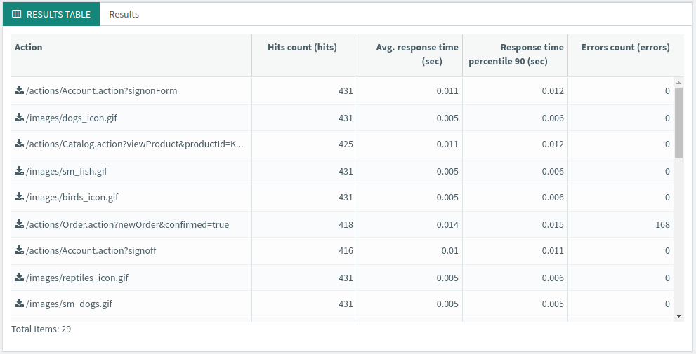
The results table provides global statistics per transaction or request.

Thresholds

The thresholds table displays the threshold warnings and errors occured during the test. Threshold are associated to the monitoring feature. Monitoring allows you to capture backend server monitoring metrics.

Top Chart

The top chart item provides a top of containers or http requests for a given metric. This chart is great for drill-down to find slow business transactions and/or requests.

Pie Chart

Pie charts are useful to get a quick overview of HTTP Response code, HTTP methods and HTTP response media types repartition. It allows to quickly spot if the web applications is running as expected.

Percentiles

Percentiles charts shows the point at which a certain percentage of observed values occur. For example, the 95^th percentile is the value which is greater than 95% of the observed values.

Errors Table

The errors table provide details about each error which occurred during the test. It allows to understand what happened server-side during the load test.

For each logged error, you can view the request sent and response received from the server.

JMeter JTL and Logs

OctoPerf lets you view JMeter logs after executing a Virtual User validation or a load test. You can also download the full log file by clicking on the Download button. A .log.gz is downloaded when you click on it. You need a file compression tool like 7Zip to extract it.

JMeter JTL files are also automatically centralised at the end of the test.

Comparison table

Guess what? We have compiled a comparison table which directly compares the Top 3 JMeter Cloud Solutions of the market:

	OctoPerf	Blazemeter	Flood.io
Recorder
HAR Import
Single URL/REST
Jmeter Import
Gatling import
Correlations		In Jmeter	In Jmeter
Variables		In Jmeter	In Jmeter
Validate script		In Jmeter	In Jmeter
Host file override
SLA
Sandbox (free unit test)	100 tests per month	10 tests only	5 hours only
Bandwidth emulation		Global only
Latency emulation		Global only
Think time		Global only	In Jmeter
Pacing
Ramp down
Hits & RPS load policy			In Jmeter
Real browser monitoring
LG startup & config	Automatic	Manual	Manual
LG monitoring
Several JMX in one test
Pre-test checks
Live filters
Duration filter
Automatic SLAs	APDEX		APDEX
Reserve IP
Default views	Good	Good	Average
Overall usability	Good	Average	Average
Collaborative access
Logs
Error details	with details
Editable graphs		one graph only
Export PDF
Export CSV	through JTL
Customize report text
Comparison
Trending
Report public link
Report availability	Unlimited	1 week to unlimited	1 to 12 months
Jmeter version	Latest Jmeter version supported	Several Jmeter versions supported	One version of Jmeter only, currently not the latest (3.1 instead of 3.3)

Summary

There are many different ways to collect and display JMeter performance metrics. From DIY open-source tools to proprietary solutions, there is a solution for everyone. Which solution should you use? Here is a brief summary.

• UI Listeners: great for debugging purpose, you can use them for very small load tests (under 50 concurrent users),
• JTL Files + Simple Data Writer: this solution can be used for distributed tests, although the configuration can be tedious. JTL files can then be analyzed using JMeter XSL sheets or via the HTML report,
• Backend Listener + InfluxDB + Grafana: This solution eliminates the tedious work of gathering and merging JTL files in distributed testing. It also provides live metrics during the test. But the setup is difficult, requires advanced knowledge and multiple systems must be maintained,
• Saas Solutions: Easiest and most powerful solution, but you have to pay for tests larger than 50 concurrent users on most platforms. You can potentially save a huge amount of time on test setup and results analysis.

The chosen solution highly depends on the following factors:

• Time: is the load testing phase tight on time?
• Budget: is there a budget being allocated to cover the load testing expenses? How much is the budget?
• Expertise: How much expertise in the load testing field do you have?

Open-source and DIY solutions are usually free but cost a lot of time. Proprietary solutions have a cost but are way more time effective. Whether you have time, budget or even both, there is a solution for everyone.

Bookshelf

If you would like to master JMeter, we would like to recommend you some good books about JMeter.

Learn JMeter In One Day, Krishna Rungta

The book starts with an introduction to Jmeter and performance testing. Gives details steps to install Jmeter on various platforms. It proceeds to familiarize the reader with the Jmeter GUI. Then the book teaches to create performance test and enhance the test using Timer, Assertion, Controllers, and Processor.

JMeter CookBook, Bayo Erinle

Leverage existing cloud services for distributed testing and learn to employ your own cloud infrastructure when needed. Successfully integrate JMeter into your continuous delivery workflow allowing you to deliver high quality products. Test application supporting services and resources including RESTful, SOAP, JMS, FTP and Database.

Want to become a super load tester?

Request a Demo